
The Coin Toss Bet
There are two possible outcomes in a coin toss bet: you either win or lose. If you lose then you forfeit the entire amount that you bet, and if you win you get back some multiple of your bet. To analyze this, we need to define the following variables:
an = the amount of money you have going into the nth bet. a0 is the amount of money that you start with.
bn = the amount of money you bet on the nth bet.
α = the multiple of your bet that you receive if you win (must be greater than 1).
p = probability of winning the bet.
q = 1 - p = probability of losing the bet.
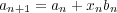
After the nth bet, your an+1 will be one of two values.
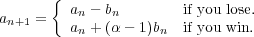
This can also be written as follows
 | (1) |
where xn is a random variable with distribution
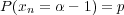 | (2) |
 | (3) |
So the question now is, how should we select the amounts to bet? One simple method is to bet a fixed fraction of the amount of money you have at the beginning of each bet. Let f be the fraction, then the bet amount will be
 | (4) |
Now if you substitute this into eq. 1 you get
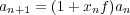 | (5) |
This is what is known as a first order stochastic difference equation. You can easily iterate it so as to express an in terms of your initial money a0 and the random variables xn. Doing this gives
 | (6) |
Alternatively, an can be expressed in terms of the random variable w which is the number of wins in a series of n bets. This expression for an is
 | (7) |
w is a binomial random variable with a distribution given by
 | (8) |
The mean or expected value of w is
![E [w ] = np](cointoss9x.png) | (9) |
and the variance is
![Var[w ] = E[w2]- E2[w] = npq](cointoss10x.png) | (10) |
For large n, the binomial distribution can be approximated by a Gaussian or normal probability density function
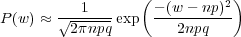 | (11) |
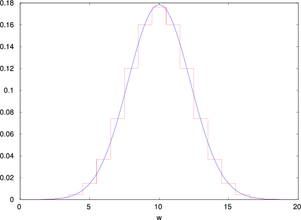
Fig. 1 shows a plot of P(w) and the normal approximation for n = 20, p = 0.5. Even for this relatively small value of n the agreement is quite good. The probability that w is less than or equal to some value W is
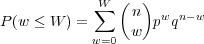 | (12) |
or in terms of the normal approximation
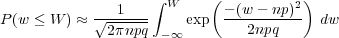 | (13) |
These formulas for the win probabilities will be used later when we look at the probabilities of an reaching different values. Now we want to look at the problem of choosing the optimal betting fraction f.
We’ll start by looking at the expected value of an. The expected value can be calculated using any of the previous equations for an. Using the recursion equation for an gives
![E[an+1] = E[(1+ xnf)an] = E[1+ xnf]E [an]](cointoss15x.png) | (14) |
![E [1 +xnf ] = (1+ (α- 1)f)p+ (1- f)q = (1+ f(αp - 1))](cointoss16x.png) | (15) |
![E [an+1] = (1 +f (αp - 1))E [an]](cointoss17x.png) | (16) |
With E[a0] = a0 this recursion equation can be written as
![E [an] = (1+ f (αp - 1))na0](cointoss18x.png) | (17) |
From this equation you can see that the expectation will only grow with n if the f(αp - 1) term is positive. This means that the probability must obey
 | (18) |
A bet for which this is true is called a positive expectation bet. Note that if p = 1∕α then eq. 17 reduces to E[an] = a0 which means that you will on average end up with as much as you started. This is called a fair bet. If p < 1∕α then you will be raising a number less than 1 to the power n in eq. 17 which means the expectation will decrease with n and your starting amount, a0, will slowly dwindle away. This is called a negative expectation bet. This is the kind of bet you will most often encounter when playing casino games. No matter how lucky you feel, it is best to stay away from this kind of bet.
Now if you try to select f based solely on eq. 17 you would conclude that it is best to make f as large as possible. Indeed why not just set f = 1. This would be a mistake. With f = 1 you are betting your entire bankroll on every bet. This only makes sense if you have no probability of losing, meaning p = 1 and q = 0. If q≠0 then it will take just a single loss to ruin you. Choosing an f < 1 is clearly the best way to go. But exactly what value of f is optimal?
We can go about choosing an optimal f in a number of different ways. Perhaps the most obvious thing to do is try to find the maximum of an with respect to f. Equivalently, we could try to maximize log(an). This is mathematically more convenient, so let’s give it a try. Using eq. 7, we can express log(an) as follows1
 | (19) |
Setting the derivative of this with respect to f, equal to zero, and then solving for f gives
 | (20) |
For this to be a maximum of log(an), the second derivative evaluated at f = fm should be negative. The second derivative evaluated at fm is
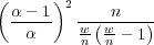 | (21) |
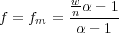
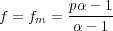
For w < n, this expression will be negative, so that fm does maximize an. For w = n, fm = 1 and an = αn. This of course makes sense, if you know you’re going to win every bet, then you should bet all you have on each bet and your money will increase by a factor of α with each bet. The problem is you have no way of knowing beforehand how many wins you will get in n bets. So what use is eq. 20? Short of being clairvoyant, all you can do is use the expected value of w which is pn. This will give you a betting fraction equal to
 | (22) |
A calculator for this formula is on a separate page. This betting fraction may not give you the maximum possible value of an but it will maximize the expectation of log(an) as we will now show.
Start by taking the log of eq. 6 which can then be written as 2
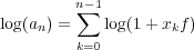 | (23) |
The expectation is
![n-1
E [log(an)] = ∑ E [log(1+ xkf)]
k=0](cointoss25x.png) | (24) |
where
![E [log(1 + xkf)] = plog(1+ (α - 1)f) + qlog(1- f)](cointoss26x.png) | (25) |
so that
![-
E[log(an)] = n(plog(1 +(α - 1)f )+ qlog(1- f)) = nr](cointoss27x.png) | (26) |
where r is the mean exponential growth rate and is defined as
 | (27) |
Maximizing r with respect to the betting fraction f, will maximize the expectation of log(an). The derivative of r with respect to f is
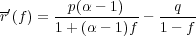 | (28) |
Setting this equal to zero and solving for f gives
 | (29) |
Note that this is the same as eq. 22. To test whether this is a maximum or minimum, look at the second derivative of r evaluated at f = fm
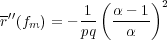 | (30) |
Since this is negative, r(fm) is a maximum. The fraction f = fm is called the Kelly fraction. Betting this fraction of your bankroll on each bet will maximize the expectation of log(an).
The expression for the maximum value of r can be written as
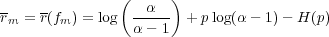 | (31) |
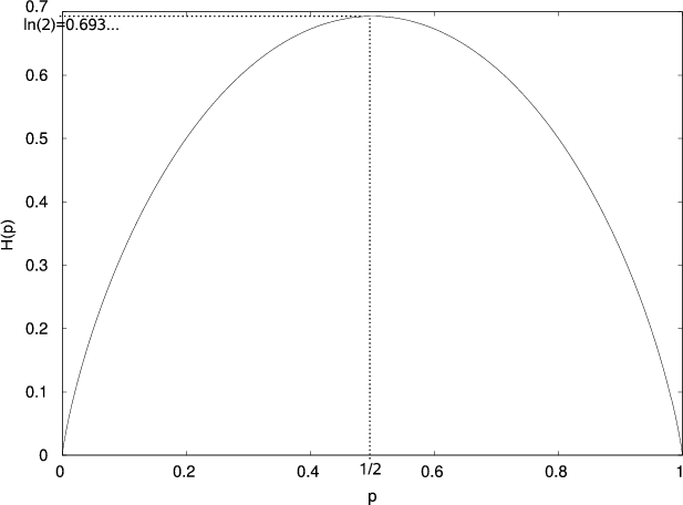
where H(p) is the binary entropy function defined as
 | (32) |
A plot of this function is shown in Fig. 2.
Assets greater than A after n coin toss bets
Now let’s look at the probability that your bankroll is greater than or equal to some value A after a given number of bets. In other words, we want to know what is the probability that an ≥ A for some given n? Using eq. 7
 | (33) |
Solving this equation for w gives
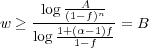 | (34) |
From which you can see that finding the probability that an ≥ A is equivalent to finding the probability that w ≥ B.
 | (35) |
The probability of having w wins in n bets is given by eq. 8, therefore we have
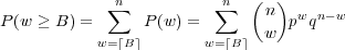 | (36) |
Fig. 3 shows a plot of this expression versus n, for A = 2, α = 2, p = 0.6, f = 0.2, and n = 1…100.
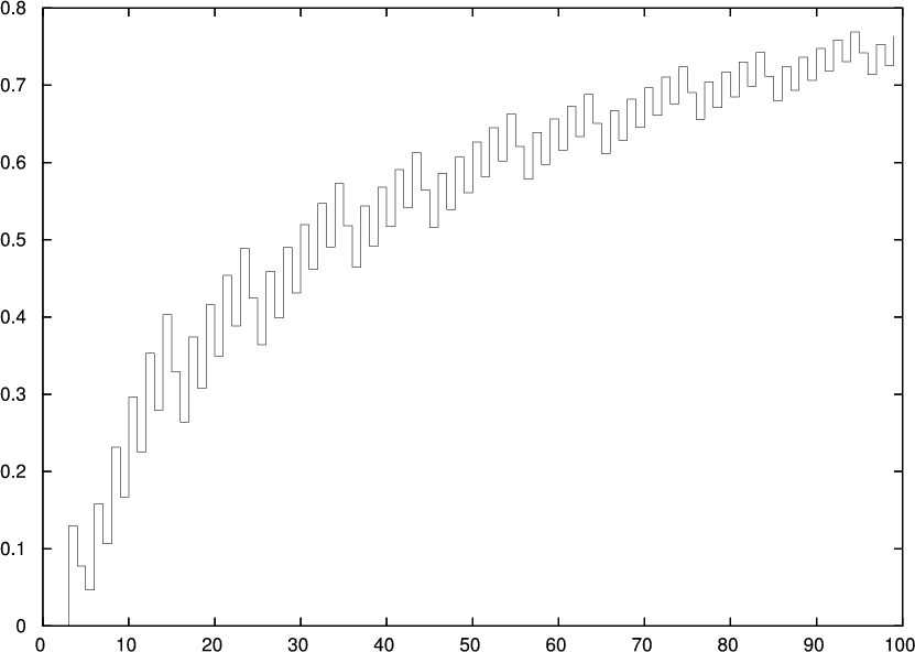
Notice the curious property that P(an ≥ A) sometimes goes down as n increments by 1. This is due to the discrete nature of the betting, where some an values might be very close to A but still less than A.
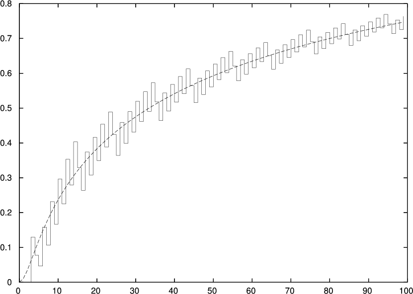
Fig. 3 is more misleading than illuminating. If we approximate the discrete distribution of w by the continuous distribution in eq. 11 then we get
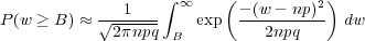 | (37) |
Fig. 4 shows the continuous version alongside the discrete one. The continuous version gives a better idea of how probabilities change as n increases.
Another way to circumvent the misleading nature of Fig. 3 is to ask a similar, but different question: What is the average amount by which you would be above A after n bets? This average is given by
 | (38) |
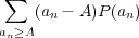
This is equivalent to the sum
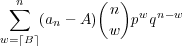 | (39) |
where B is given by 34. Fig. 5 shows a plot of this versus n, for A = 2, α = 2, p = 0.6, f = 0.2, and n = 1…100.
|
|
Notice the constant upward growth as n increases, so the average amount by which you would be above A after n bets, always goes up.
Calculating the probability that an is less than some value A is very similiar to what we did above.
Next we will show some simulations of coin toss betting using the Kelly fraction.
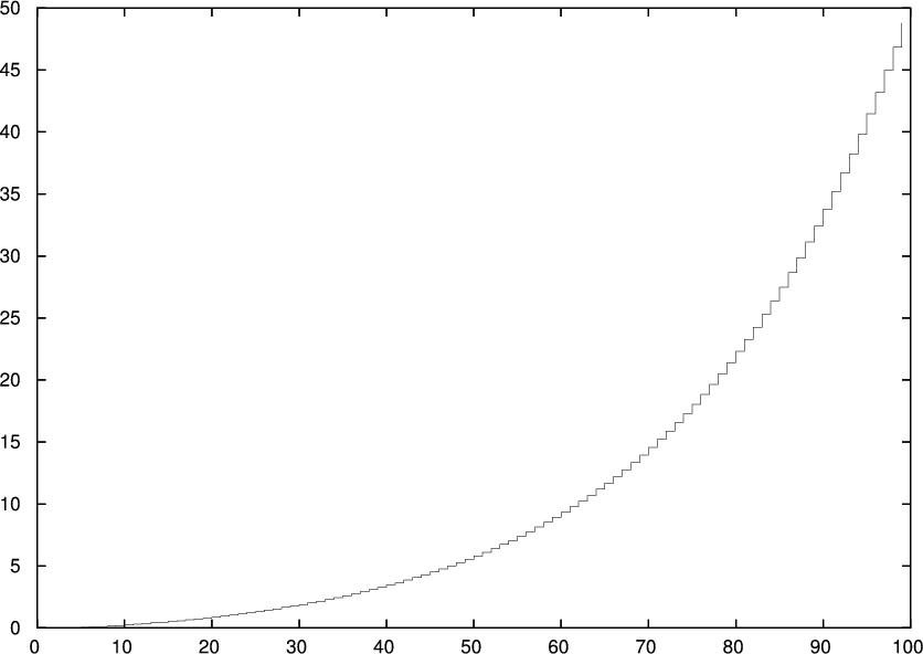
Coin toss bets with Kelly fraction
The two non-straight lines in Fig. 6 are log(an) for a series of coin toss bets, with α = 2, p = 0.6, and f = 0.2, which is the Kelly fraction for this α and p. The smoother of those two lines is an average of 2000 runs. The straight line is log(E[an]) with α, p, and f, the same.
|
|
References
[1] S.N. Ethier. The kelly system maximizes median fortune. Journal of Applied Probability, 41(4):1230–1236, dec 2004.
[2] S.N. Ethier and S. Tavar. The proportional bettor’s return on investment. Journal of Applied Probability, 20(3):563–573, sept 1983.
[3] J.L. Kelly. A new interpretation of information rate. The Bell System Technical Journal, 35:917–926, july 1956.
[4] William Poundstone. Fortune’s Formula: The Untold Story of the Scientific Betting System that Beat the Casinos and Wall Street. Hill and Wang, 2005.
[5] E.O. Thorp. Optimal gambling systems for favorable games. Review of the International Statistical Institute, 37(3):273–293, 1969.
[6] E.O. Thorp. The Mathematics of Gambling. Gambling Times, 1985.
[7] E.O. Thorp. The kelly criterion in blackjack sports betting, and the stock market. Handbook of Asset and Liability Management, Volume 1, 2006.
[8] Stanford Wong. What proportional betting does to your win rate. Blackjack World,, 3:162–168, 1981.
[9] Rachel E. S. Ziemba and William T. Ziemba. Optimal gambling systems for favorable games. Proceedings of the Fourth Berkeley Symposium on Mathematical Statistics and Probability, I:65–78, 1961.